SambaFlow Developer Guide
Copyright © 2020-2023 by SambaNova Systems, Inc. All contents are subject to a licensing agreement with SambaNova Systems, Inc. Any disclosure, reproduction, distribution, reverse engineering, or any other use made without the advance written permission of SambaNova Systems, Inc. is unauthorized and strictly prohibited. All rights of ownership and enforcement are reserved.
- SambaFlow software release notes
- Hello SambaFlow! Compile and run a model
- Architecture and workflows
- Transition to DataScale SN30
- Examine logreg model code
- Convert a simple model to SambaFlow
- Run language example applications
- Using LayerNorm instead of BatchNorm
- How to use data parallel mode
- What is data parallel?
- How does SambaFlow use data parallel operations?
- Modify an application to work in data parallel mode
- Compile a data parallel application
- Run a data parallel application
- Data parallel best practices
- Data parallel example command
- Data parallel mode and tensor parallel mode
- Resources
SambaFlow software release notes
Release 1.23
Release 1.23 includes improved OS support, changes to application locations, and renaming of components. Please review the following updates carefully to ensure compatibility with your environment.
Supported OS versions
-
Red Hat: Starting with this release, SambaFlow supports Red Hat (8.8).
-
Ubuntu: The version for Ubuntu 22.04.x remains unchanged.
Package/Application location change
To align with Linux best practices, 3rd party applications have been relocated from their previous locations (/opt/ or /usr/local/) to a more standardized directory (/opt/sambanova/). This change ensures compatibility, avoids conflicts with pre-installed customer packages, and provides controlled versions compatible with the SambaNova software stack.
-
New location:
/opt/sambanova/ -
Previous locations:
/opt/and/usr/local/
If you rely on custom scripts or configurations pointing to old paths, please update references to the new directory.
Renamed applications
The following applications have been renamed, and their old names are deprecated starting with release 1.23.
| Old names (deprecated) | New names |
|---|---|
|
|
|
|
|
|
Release 1.21
Release 1.21 includes internal code changes that support our first release of SambaNova Model Zoo, available in this public GitHub repository.
This first official release of SambaNova Model Zoo is currently in Beta. SambaNova customers can download a container image (Devbox) that includes the SambaFlow compiler, other SambaNova libraries, and all prerequisite software.
-
Existing SambaNova customers can contact their Customer Support representative to access the Devbox.
-
If you’re new to SambaNova and interested in trying out Model Zoo, contact us at help@sambanovasystems.com to get started!
See the Model Zoo Release Notes for details.
Release 1.20
Release 1.20 was an internal release. No user-visible changes were made in that release.
Release 1.19
New features
This release has primarily had a focus on performance improvement and some other features that are not yet visible to customers.
Cached compilation mode (experimental)
Our experimental cached compilation mode can speed up compilation times of large models. In this mode, the compiler maintains a cache of previously compiled sections of a model, so that subsequent compilations can use the cached sections instead of recompiling them.
-
To enable cached compilation mode, set the
SN_PEF_CACHEenvironmental variable to the path of a folder. -
The compiler will then populate a cache at that location (and create the folder if it doesn’t exist). The content of the cache is an internal detail subject to change.
| Cached compilation mode supports the development flow of a single user who makes frequent changes to a model. You cannot share the cache with other users. For the best use of the cache, make small changes (instead of extensive changes) followed by a compile. By limiting the scope of a change, you increase the likelihood that more sections can be pulled precompiled from the cache because they did not change. |
API updates
-
In
argmax(), the default value ofkeepdim (bool)has changed fromTruetoFalse.keepdimis used to indicate whether Samba retains the dim in the output tensor. Now the dim is no longer retained by default. -
The
groupby()operator was added in this release.
Release 1.18
In Release 1.18, most of SambaFlow was migrated from /usr/local to /opt/sambanova. Add /opt/sambanova/bin to your PATH. s
|
New features
-
Tensor parallel support (Beta). Tensor parallel mode uses multiple RDUs for inference and training. Tensor parallel speeds up the runtime performance and ensure that large models, which might exceed the memory limit of a single socket, still run. See How to use tensor parallel mode (Beta) for details.
-
Multigraph support. The new multigraph feature supports partitioning a model into individual graphs so you can run each graph separately. See Use multigraph to partition models.
-
UE Replay (Beta). Some updates to Uncorrectable Error replay (Beta) make the feature easier to use.
-
Mixed precision (Beta). Mixed precision combines the use of different numerical formats (such as FP32 and BF16) to reduce memory footprint and speed up large neural network workloads. See Mixed precision support for details and examples.
Compiler and performance improvements
-
New and renamed heuristics. This release includes improvements to heuristics for use with o1.
-
SAFE_GEMM,DEFAULT_GEMM(new),AGGRESSIVE_GEMM. Applicable only to patterns that are dominated by a single large matrix multiply (GEMM) operation. -
MHA(renamed in 1.18). For use with a multi-headed attention block. Renamed from GPT3_MHA. -
SDPA(new in 1.18). For use with PyTorch SDPA operations.
-
-
The compiler’s new deduplication feature can reduce compile time and improve model performance. The feature is currently limited to a single RDU. The feature is on by default. Contact Customer Support if you see a need to turn it off.
-
This release includes an improved algorithm for mapping compute graphs onto RDU resources. The enhanced algorithm, which is on by default:
-
Accelerates the optimization process, resulting in shorter compile times
-
Reduces on-RDU congestion when running models, providing performance improvements.
-
New operators
This release includes several new PyTorch operators. See Functional Operators ![]()
| Supported datatypes for each new operator are still being validated and more information will be made available at a later date. If you have specific questions on support datatypes, contact SambaNova Support. |
-
Arithmetic operators
-
abs() -
mul() -
relu() -
rsqrt() -
scale() -
sigmoid() -
silu()
-
-
Parallel patterns operators
-
sn_gather() -
sn_imm() -
sn_iteridx() -
sn_reduce() -
sn_scatter() -
sn_select() -
sn_zipmapreduce()
-
-
Tensor operators
-
ct_attention() -
sn_identity() -
to() -
type_as()
-
-
Other operators
-
multi_head_attention() -
layer_norm()
-
Documentation improvements
-
Updated SambaFlow API Reference
 with a new template that supports both dark and light mode.
 -
In the API reference, new APIs now include information about the release (e.g. New in 1.18)
-
Updates to the _Run pretrained models on RDU tutorial- include code snippets for download and conversion of the dataset in hf-compile-run.adoc#_download_the_dataset and hf-compile-run.adoc#_prepare_the_dataset.
Release 1.17
New compiler features
-
Released o0 and o1 compiler optimization modes (previously in Beta). See Compiler optimization modes.
-
(Beta) Added support for operator fusion rule yaml files and heuristics for use in conjuction with the o1 compiler option.
-
SambaNova will make a limited set of fusion rule yaml files available that direct the compiler, resulting in a more highly optimized PEF for certain families of models (e.g. LLM). See Operator fusion rule yaml syntax.
-
Users can make changes to the yaml file to achieve more efficient compiler behavior.
-
-
(Beta) Added support for preset scheduling heuristics to improve fused operators' performance in o1 compiler mode. Users cannot edit the heuristics in this release. See Operator fusion heuristics.
Other new features and improvements
-
Introduced beta version of the uncorrectable error replay (UE replay) feature, which attempts to automatically recover and continue a training run if the run encounters a UE. See Uncorrectable Error replay (Beta).
-
For improved performance, changed ENABLE_LINEAR_GRAD_ACCUM_STOC to default to 1 instead of 0. As a result, stochastic rounding is turned on for mixed-precision general matrix multiply (GEMM) by default. If you want to return to the previous default, contact SambaNova Support.
-
Enhanced PyTorch operator support
-
silu: FP32 (experimental support) -
gelu: FP32 (experimental support) -
tanh: FP32 (experimental support) -
For
mul, full support for B16 and FP32 had been omitted from the documentation by mistake. It’s now been added.
-
Performance improvements
-
Enabled compile-time device-program control scheduling for Bloom 176B and GPT13B LLM models for NLP inference.
Documentation improvements
| Some documentation updates that are not release dependent became available in the SambaFlow 1.16 documentation after that version was released. Here is the complete list of release-dependent and release-agnostic documentation. |
-
Several of our tutorials are now available from the new sambanova/tutorials
GitHub repo. More to be added in future releases. See Tutorials for an overview of all tutorials. -
SambaFlow learning map has an overview of documentation and tutorials for new users.
-
Model conversion overview is a high-level discussion of model porting tasks. Includes pointers to the porting example that is part of this doc set.
-
Hyperparameter reference is a short overview of Hyperparameters. We’ll point to that doc page from session:run() in the API reference
. -
Updates and fixes in Compiler argument reference.
API Reference improvements
Changes and additions to the SambaFlow API reference ![]() :
:
-
Added documentation for
samba.random -
Added documentation for
samba.from_torch_model -
Added documentation for
samba.utils.trace_graph -
Added documentation for
samba.optim -
Fixes to some supported data types in
Functional Operators -
Small fixes for
samba.sessiondocumentation -
Fixed some broken links
Release 1.16 (2023-07-14)
New features and other improvements
-
Introduced new compiler modes -o0 and -o1 (Beta), which allow users to fine-tune compiler performance.
-
See SambaFlow compiler overview for some background information.
-
See Compiler argument reference for reference documentation, which includes examples.
-
-
Change to compiler
--helpbehavior. The--helpcommand now returns a limited number of fully supported options. A call to compile with--help --debugreturns a longer list of options, some of them experimental.
Performance improvements
-
Various optimizations in this release help improve model performance and reduce compile times especially for NLP models.
Documentation improvements
-
Updated API Reference includes documentation for supported PyTorch operators
API Reference documentation always opens in a new tab (or window). To return to the main doc set, click the previous tab (or window). -
New SambaNova messages and logs doc page explains which messages you can safely ignore, where to find which logging information, and which errors you might be able to resolve yourself.
-
New SambaFlow compiler overview doc page gives an overview of the compiler stack and discusses some compiler arguments, including the new o0, o1, etc. options.
-
New Compiler argument reference doc page is a reference to frequently used compiler arguments and includes a discussion of the new arguments.
-
New Use sntilestat for performance analysis doc page explains how to use the
sntilestattool for performance analysis and includes examples of visualizingsntilestatCSV output in a spreadsheet.
Release 1.13 (2022-11-03)
New features and other improvements
-
New features
-
Added option to
sntilestatto skip idle tiles. -
Enhanced multi-processing support for SambaNova Runtime APIs.
-
Enhanced host profiling information and detailed timeline view in SambaTune.
-
Enhanced
snprofand added more robust fault reporting insnstat.
-
-
Performance improvements
-
Faster SambaFlow context creation.
-
More efficient CPU usage.
-
Better performance for scaleout operations.
-
-
Software
-
Updated PEF to version 2.5.0.
Recompile all models with this release due to the PEF version change. -
Version 2 of SambaFlow compiler scheduler, specified with option
--mac-v2, is now the default. The--mac-v1is still supported but requires using explicit option.
-
Deprecated components
-
venv: The
venvshared generic package is deprecated and has been replaced by model-specificvenvpackages. The generic package will be removed from future releases. -
UnoSecInf: The UnoSecInf inference performance test, which is based on section-by-section mapping, is deprecated starting in Release 1.13. Starting in Release 1.14, this performance test will no longer be available.
The
uno_full.pymodel is not deprecated.
Release 1.12.7 (2022-07-30)
New features
-
Added SambaTune: a tool that supports profiling application performance.
-
Improved Scale-out performance through parallel reduce.
-
Enhanced RDU reset support with VM.
Supported components and versions
Hello SambaFlow! Compile and run a model
Welcome! In this tutorial, you learn how to compile and run a logreg.py example model. This Hello SambaFlow! example uses the classic machine learning problem of recognizing the hand-written digits in the MNIST dataset.
In this tutorial you:
-
Ensure that your environment is ready to compile and run models.
-
Compile the model to run on the RDU architecture. Compilation generates a PEF file.
-
Do a training run of the model, passing in the generated PEF file.
| We discuss the code for this model in Examine logreg model code. |
Prepare your environment
To prepare your environment, you ensure that the SambaFlow package is installed.
Check your SambaFlow installation
You must have the sambaflow package installed to run this example and any of the tutorial examples.
-
To check if the package is installed, run this command:
-
For Ubuntu Linux
$ dpkg -s sambaflow -
For Red Hat Enterprise Linux
$ rpm -qi sambaflow
-
-
Examine the output and verify that the SambaFlow version that you are running matches the documentation you are using.
-
If you see a message that
sambaflowis not installed, contact your system administrator.
Download the model code
Before you start, clone the SambaNova/tutorials GitHub repository, as instructed in the README.
After a SambaFlow upgrade, you might have to do a git pull again if your model no longer works.
|
Compile and run your first model
To compile and run your first model, you check supported options, prepare data, and then run scripts to compile and run logreg.
Look at supported options
Each example and each model has its own set of supported options, so it’s important to list them explicitly.
To see all arguments for the logreg model, change to the directory you created earlier and look at the --help output:
$ cd $HOME/tutorials/logreg
$ python logreg.py --help
The output looks similar to the following, and shows that you can compile and run this model.
usage: logreg.py [-h] {compile,run,test,measure-performance} ...

positional arguments:
  {compile,run,test,measure-performance}
                        different modes of operation

optional arguments:
  -h, --help            show this help message and exit
The test and measure-performance options are primarily used internally or when working with SambaNova Support.
|
You can drill down and run each command with --help to see options at that level. For example, run the following command to see options for run:
$ python logreg.py run --help| In most cases, using the defaults for the optional arguments is best. In Useful arguments for logreg.py we list a few commonly used arguments. |
Prepare data
This tutorial downloads train and test datasets from the internet, so there’s no separate step for preparing data.
If your system does not have access to the internet, download the data to a system that has access and make the files available. See Download model data (Optional).
Compile logreg
When you compile the model, the compiler generates a PEF file that is suitable for running on the RDU architecture. You later pass in that file when you do a training run.
-
Start in the
tutorials/logregdirectory that you created in Create your own directory.$ cd $HOME/tutorials/logreg -
Run the compilation step, passing in the name of the PEF file to be generated. You will later pass in that file when you do a training run.
$ python logreg.py compile --pef-name="logreg" -
The compiler runs the model and displays progress messages and warnings on screen.
-
You can safely ignore all
infoandwarningmessages. -
If a message says
warning sambait might indicate a problem with your code. -
For some background, see SambaNova messages and logs.
-
-
When the command returns to the prompt, look for this output, shown toward the end:
-
Compilation succeeded for partition_X_Xshows you that compilation succeeded. -
Logs are generated in …shows where the log files are located.
-
-
Verify that the PEF file was generated:
$ ls -lh ./out/logreg/logreg.pefThe generated PEF file contains all information that the system needs to do a training run of the model.
Start a logreg training run
When you do a training run, the application uploads the PEF file onto the chip and trains the model with the specified dataset. This example uses the MNIST dataset. The example code downloads the data set automatically.
| If your system is disconnected from the Internet you have to manually download the dataset to a system with Internet access and copy the dataset to the system you are running the models on. See Download model data (Optional). |
-
Start a training run of the model with the PEF file that you generated. Use
-eto specify the number of epochs (default is 1).$ python $HOME/sambaflow-apps/starters/logreg/logreg.py run --num-epochs 2 --pef=out/logreg/logreg.pefEven one epoch would be enough to train this simple model, but we use
--num-epochsto see if loss decreases in the second run. The run command:-
Downloads the model data.
-
Returns output that includes the following:
2023-01-25T15:14:06 : [INFO][LIB][1421606]: sn_create_session: PEF File: out/logreg/logreg.pef
Log ID initialized to: [snuser1][python][1421606] at /var/log/sambaflow/runtime/sn.log
Epoch [1/2], Step [10000/60000], Loss: 0.4634
Epoch [1/2], Step [20000/60000], Loss: 0.4085
Epoch [1/2], Step [30000/60000], Loss: 0.3860
Epoch [1/2], Step [40000/60000], Loss: 0.3702
Epoch [1/2], Step [50000/60000], Loss: 0.3633
Epoch [1/2], Step [60000/60000], Loss: 0.3555
Test Accuracy: 91.54  Loss: 0.3012
Epoch [2/2], Step [10000/60000], Loss: 0.2861
Epoch [2/2], Step [20000/60000], Loss: 0.3065
Epoch [2/2], Step [30000/60000], Loss: 0.3080
Epoch [2/2], Step [40000/60000], Loss: 0.3084
Epoch [2/2], Step [50000/60000], Loss: 0.3076
Epoch [2/2], Step [60000/60000], Loss: 0.3061
Test Accuracy: 91.54  Loss: 0.3001
-
Congratulations! You have run your first model on the SambaNova system! The output shows that the training run is successful and has a very low loss percentage, which decreases over time.
Useful arguments for logreg.py
Each of the example model commands has several arguments. In most cases, the default gives good results.
Arguments for compile
For a list of compile arguments for use with logreg.py, run this command:
$ python $HOME/tutorials/logreg/logreg.py compile --helpThe command returns a full list of arguments. Here are some useful arguments:
-
--pef-name— Name of the output file, which has the information for running the model on RDU. -
--n-chips,--num-tiles— Number of chips you want to use (from 1 to 8) and the number of tiles on the chip (1, 2, or 4). Default is 1 chip (4 tiles). -
--num-features— Number of input features (for this model the default is 784) -
--num-classes— Number of output labels (for this model the default is 10)
Arguments for run
For a list of run arguments for use with logreg.py, run this command:
$ python $HOME/tutorials/logreg/logreg.py run --helpThe command returns a full list of arguments. Here are some important arguments:
-
-p PEFThe only required argument. A PEF file that was the output from a compile. -
-b BATCH_SIZE, --batch-size BATCH_SIZE— How many samples to put in one batch. -
-e,--num-epochs— How many epochs to run with the model. -
--num-features,--num-classes— Input features and output classes for the model. -
--lr— Learning rate parameter. Decimal fraction between 0 and 1.
Learn more!
-
See SambaNova messages and logs to understand what the messages to stdout mean.
-
See Use Python virtual environments to learn how to run models inside a Python virtual environment.
-
See Compilation, training, and inference for an intermediate tutorial that includes using checkpoints and running inference.
-
Find other tutorials in our SambaNova Tutorials public GitHub repo
. See Tutorials:GitHub and doc for an overview.
Download model data (Optional)
| Only users without internet access perform this task. By default, the application code downloads model data. |
If you run the example on a system that is not connected to the internet, you have to download the model data from a connected system and copy the data to the system where you want to run the model.
-
On a connected system run:
$ mkdir -p /tmp/data/MNIST/raw $ cd /tmp/data/MNIST/raw $ wget http://yann.lecun.com/exdb/mnist/train-images-idx3-ubyte.gz $ wget http://yann.lecun.com/exdb/mnist/train-labels-idx1-ubyte.gz $ wget http://yann.lecun.com/exdb/mnist/t10k-images-idx3-ubyte.gz $ wget http://yann.lecun.com/exdb/mnist/t10k-labels-idx1-ubyte.gz -
Copy the four
.gzfiles to the DataScale system and place them in the directory/tmp/data/MNIST/raw. -
When you later use the
compileand theruncommand, add the--data-folder=/tmp/dataargument.
Architecture and workflows
The SambaFlow™ software stack runs on DataScale® hardware. You can run models on this software stack in several ways:
-
To get started, use the tutorials available from the SambaNova tutorials repo. You can also examine and compile and run models included in
opt/sambaflow/appson your DataScale host. -
To progress, use one of the models available in the SambaNova modelzoo repo. You run Model Zoo models in a DevBox container that includes all prerequisite software. The model source code, which been customized for RDU, is available in a public GitHub repo, which also includes example apps. You can compile a model, and can then run inference (text generation) and fine-tune the model with custom data. To fine tune, you download a checkpoint for the same model (Hugging Face format), prepare your dataset, and compile and train the model.
In this doc page, you learn about the different components of the software stack, the compile/train and compile/generate cycles, and the command-line arguments.
SambaNova Stack
It’s useful to understand the different components of the SambaNova hardware and software stack and how they interact with each other. For example, SambaFlow developers might find it useful to investigate what’s going on in the SambaNova Runtime component.
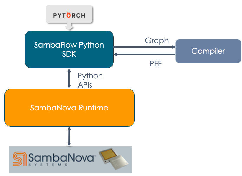
-
SambaNova Reconfigurable Dataflow Unit™ (RDU) is a processor that provides native dataflow processing. It has a tiled architecture that consists of a network of reconfigurable functional units. See the white paper SambaNova Accelerated Computing with a Reconfigurable Dataflow Architecture
. -
SambaNova Systems DataScale is a complete rack-level computing system. Each DataScale system configuration consists of one or more DataScale nodes, integrated networking, and a management infrastructure in a standards-compliant data center rack.
-
SambaNova Runtime. The SambaNova Runtime component loads code and data onto the RDUs and manages the return of result data. System administrators can perform configuration, fault management, troubleshooting, etc. See the SambaNova Runtime documentation for details.
-
SambaFlow Python SDK. The SambaFlow Python SDK serves as our frontend for compiling and running models on SambaNova hardware.
-
SambaFlow models. We offer models in several places.
-
Starter models are included on the SambaNova host at
/opt/sambaflow/apps/and are targeted towards the new user. -
SambaFlow models in our sambanova/tutorials
GitHub repo allow you to examine the Python code and then perform compilation, training, and inference runs. See SambaFlow tutorials. -
Model Zoo, available from the public modelzoo repo includes model source code that’s been customized to work well on RDU, and scripts for running them. You run the models in a Devbox container. You can use Model Zoo in conjunction with checkpoints in Hugging Face format (and a corresponding config.json) to fine tune the model with your data.
-
Workflows
When you develop for RDU hardware, you start with model code, optional checkpoints, and fine-tuning data. You end with a trained model that might for example, responds to prompt data.
Data preparation workflow
It’s possible to start by training from scratch with large data sets, but it usually makes sense to work with an existing checkpoint and fine-tune that checkpoint with your own data. In both cases, your data needs to be in a format that SambaFlow can work with.
| Data preparation is a much-discussed topic in AI. This doc page doesn’t go into data preparation details but focuses instead on the format of the data, not the content. |
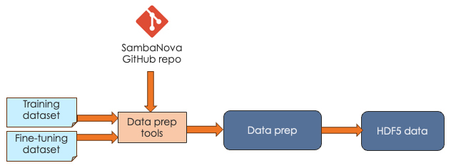
SambaNova expects that you pass in your data as HDF5 files. Our public generative_data_prep repo ![]() includes scripts and documentation for converting plain text or jsonline format files to HDF5 format.
includes scripts and documentation for converting plain text or jsonline format files to HDF5 format.
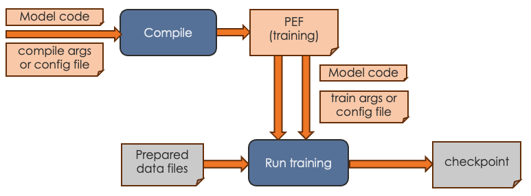
Training workflow
The goal of the training workflow is to generate a a checkpoint that you can then use in a generation workflow.
-
First you compile for training and generate a PEF file. The PEF file defines the dataflow graph for the SambaNova hardware.
-
Then you run training with the data of your choice and pass in the PEF file.
| With the small tutorial models, you can complete a training run. For the much larger Model Zoo models, we recommend that you download a checkpoint from Hugging Face and run training with your model source, the checkpoint, and your custom data instead. |
For the training workflow, you proceed as follows:
-
Complete data preparation, discussed in Data preparation workflow
-
Perform compilation by running the compilation command, passing in the model code and arguments.
-
If you’re using the container-based Model Zoo solution, you specify most arguments in a YAML config file and specify only a few on the command line.
-
If you’re using one of the tutorial examples, you specify all arguments on the command line. See Compiler argument reference.
The output of the compilation step is a PEF file, which defines how the model is run on SambaNova hardware. You cannot edit a PEF file.
-
-
Perform training by running the training command, passing in the PEF file, the configuration info for training, and the prepared data files.
-
If you’re using the container-based Model Zoo solution, you specify most arguments in a YAML config file and specify only a few on the command line. Because Model Zoo models are large models, you typically pass in a check point that you download from Hugging Face. Training a model from scratch without a checkpoint takes a long time. See the examples README for a walkthrough example with Llama2.
-
If you’re using one of the tutorial examples, you specify all arguments on the command line. Run the training command with
--helpto see all arguments.As part of a training run, information about loss and accuracy are logged to stdout.
-
-
Examine the loss and accuracy information, which is logged to stdout as part of a training run.
-
If you’re running a Model Zoo model, observe the output. If you see that loss is decreasing, your PEF is valid. You can then perform fine tuning with your own data and a Hugging Face checkpoint.
-
If you’re running a tutorial example, you can run training to completion. The output is a checkpoint file that you can use for fine tuning.
-
Fine-tuning workflow
The most common use case for SambaNova customers is to start with an existing model, generate a PEF file, fine-tune the model with custom data, and then use the model for generative inference. The workflow looks like this:
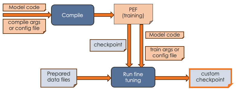
During fine tuning, you create a version of the model that’s been trained with your organization’s data.
-
Before you start fine tuning, ensure that you have the custom data in the correct format, as discussed in Data preparation workflow.
-
Start a training run and pass in:
-
A PEF file that was the output of compilation.
-
A checkpoint. For a Model Zoo model, use a publicly available Hugging Face checkpoint. For a tutorial model, you can use a checkpoint generated by a training run.
-
The configuration parameters, either on the command line or, for Model Zoo models, in a configuration file.
-
-
Output of the fine tuning run is a model checkpoint that has been fine tuned with your custom data. You can then pass in that checkpoint when you runfine- inference (generation).
Inference (generation) run
The final step is running generative inference. In this step, you send prompt data to the trained model and the model responds to the prompt or performs summarization, identification, etc. The actual tasks your model can perform depends on the model itself.
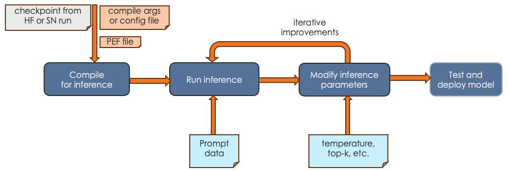
-
In most cases, you first compile an inference PEF. Compilation for inference consists only of the forward pass.
-
You run inference, passing in a checkpoint and prompt data or other input.
-
You can experiment with inference parameters, such as temperature, topk, etc. Some parameters require a recompile, others do not.
-
When you’re satisfied with the results, you can deploy the tested model.
See Run and verify inference for an example discussion.
Command-line arguments
SambaNova initially used a workflow where users passed all configuration arguments in on the command line. With our more recent Model Zoo initiative, we are using a Pydantic and Hydra infrastructure. Most arguments are specified in a YAML configuration file. A few arguments, such as the name of the PEF file, are specified on the command line.
Command-line arguments for Model Zoo models
For Model Zoo models, we have greatly simplified argument management for the developer and argument usage for the person who uses the model. A combination of Pydantic and Hydra make this possible.
-
Model developers are encouraged to become familiar with the Pydantic and Hydra infrastructure to reap the benefits of streamlined argument management.
-
Model users will notice that the scripts for running the model have a different syntax than before. For example, here’s how you might invoke generation:
/opt/sambanova/bin/python $HOME/modelzoo/modelzoo/examples/text_generation/run_rdu.py \
command=compile \
model.cache_dir=/opt/sambanova/modelbox/checkpoints \
model.batch_size=1 \
+samba_compile.target_runtime_version=1.3.7 \
+samba_compile.output_folder=/opt/out \
+samba_compile.pef_name=llama2_7b_infer
Command-line arguments for other models
For tutorial models and for models at /opt/sambaflow, each model supports different command-line arguments. To see all arguments, run the model with the task (compile or run) and --help, for example, app.py compile --help.
Compilation
-
All models support the shared arguments that are documented in Arguments to compile.
-
You can generate a PEF for inference by specifying the
--inferencecompile flag. By default, we compile for training, which includes a forward, backward, and optimization pass. Inference compilation is only a forward pass. -
All models support a shared set of experimental arguments, usually used during debugging when working with SambaNova Support. To include these arguments in the help output, run
app.py compile --debug --help. -
Additionally, each model has a set of model-specific arguments that are defined in the app code.
Transition to DataScale SN30
The DataScale SN30 system offers significantly improved performance over DataScale SN10 system. Because the system is different, you likely have to recompile and retrain a model that was compiled on SN10 system. This topic gives some guidance.
| A PEF built on SN10 is not expected to run unmodified on an SN30. |
General RDU difference information
Here are the RDU differences between SN10 and SN30.
| SN10 | SN30 |
|---|---|
8 RDUs |
8RDUs |
4 tiles per RDU |
8 tiles per RDU |
Default compile yields a PEF that uses 1 RDU (4 tiles) |
Default compile yields a PEF that uses 1 RDU (8 tiles) |
By default you run using 1 copy of the model on 1 RDU |
By default you run 2 copies of the model, one on each "half" of the RDU (using tensor parallel execution). |
Compiler impacts
RDU differences mean that the compiler optimizes the PEF file differently. Here’s what you need to know:
-
On both SN10 or SN30 you can explicitly specify the number of tiles with
num-tiles, for example,--num-tiles=4.-
If you compile with
--num-tiles=4on an SN10 system, you can run 8 instances of data-parallel on a node. -
If you compile with
--num-tiles 4on an SN30 system, you can run 16 instances of data-parallel on a node.
-
-
If you specify
--num-chips=1on SN10 or SN30 you get 4 tiles. -
Because SN30 uses tensor parallel, both compile and run operations require that the batch size be an even number. The results are reduced using data parallel in the PEF. This is the default, it is equivalent to
--tensor-parallel=batch. -
It is not unusual to need to use different human decision files and different compiler configuration files when migrating your model from SN10 to SN30.
Examine logreg model code
SambaNova supports several tutorials. You learn how to compile and train a simple logreg model in Hello SambaFlow! Compile and run a model. This doc page examines the Python code and data you’re using to run logreg.
Our logreg model uses:
-
A Python program. See the complete file in our tutorials GitHub repo at https://github.com/sambanova/tutorials/blob/main/hello_world/logreg.py.
-
A simple neural network dataset (MNIST). The example application downloads the dataset when you run the model.
In this tutorial you learn what’s inside the Python code.
What you’ll learn
This tutorial explores these topics:
-
Typical imports
-
Components of
main() -
Model definition, including input arguments, compilation, and training.
Files
All tutorial code files are in our tutorials GitHub repo at https://github.com/sambanova/tutorials/tree/main. This doc page includes collapsible code snippets for each code component we discuss.
Data
The tutorial uses the classic MNIST dataset, which includes a training set of 60,000 examples, and a test set of 10,000 examples.
-
By default, the code downloads the dataset files as part of the training run.
-
In environments that don’t have access to the internet, you can explicitly download the dataset. See (Optional) Download model data.
Imports
Our model imports several Python modules. Here’s the Python code, followed by an explanation of each import.
Imports
import argparse
import sys
from typing import Tuple

import torch
import torch.distributed as dist
import torch.nn as nn
import torchvision

import sambaflow.samba.utils as utils
from sambaflow import samba
from sambaflow.samba.utils.argparser import (parse_app_args,
                                             parse_yaml_to_args)
from sambaflow.samba.utils.dataset.mnist import dataset_transform
from sambaflow.samba.utils.pef_utils import get_pefmeta-
sambaflow.sambais the set of SambaFlow modules. -
sambaflow.samba.utilscontains all the utilities, such as tracing etc. -
parse_app_argsis our built-in argument parsing support for each supported execution mode (more details below). -
dataset_transformis a utility function to transform the data. -
get_pefmetasaves the model’s metadata in the resulting executable file (PEF file).
It all starts with main()
The workflows for SambaNova models are outlined in sambaflow-intro.adoc#_workflows[Workflows]. The intermediate tutorial includes both training and inference.
The main() function includes the functions to perform compilation and training, and also does some preparation.
| Function | Description | See |
|---|---|---|
|
Set a random seed for reproducibility while we’re in the development phases of our tutorial. |
|
|
Collect the arguments coming from |
|
|
Create random input and output for compilation |
See the API Reference. |
|
Set up the model to use the SambaFlow framework. The function, which also converts a PyTorch model to a Samba model, performs some initialization and related tasks. We pass in |
|
|
Define the optimizer we’ll use for training the model. The SambaFlow framework supports AdamW and SGD out of the box. You can also specify a different optimizer. |
See the API Reference |
|
If the user specified |
|
|
If the user specified |
Define the model
The model definition specifies the layers in the model and the number of features in each layer.
Here’s the Python code:
LogReg class
class LogReg(nn.Module):
    """ Define the model architecture

    Define the model architecture i.e. the layers in the model and the
    number of features in each layer.

    Args:
        nlin_layer (ivar): Linear layer
        criterion (ivar): Cross Entropy loss layer
    """

    def __init__(self, num_features: int, num_classes: int, bias: bool):
        """ Initialization function for this class

        Args:
            num_features (int):  Number of input features for the model
            num_classes (int): Number of output labels the model classifies inputs
            bias (bool): _description_
        """
        super().__init__()
        self.num_features = num_features
        self.num_classes = num_classes

        # Linear layer for predicting target class of inputs
        self.lin_layer = nn.Linear(in_features=num_features, out_features=num_classes, bias=bias)

        # Cross Entropy layer for loss computation
        self.criterion = nn.CrossEntropyLoss()

    def forward(self, inputs: torch.Tensor, targets: torch.Tensor) -> Tuple[torch.Tensor, torch.Tensor]:
        """ Forward pass of the model for the given inputs.

        The forward pass predicts the class labels for the inputs
        and computes the loss between the correct and predicted class labels.

        Args:
            inputs (torch.Tensor):  Input samples in the dataset
            targets (torch.Tensor): correct labels for the inputs

        Returns:
            Tuple[torch.Tensor, torch.Tensor]:The loss and predicted classes of the inputs
        """

        out = self.lin_layer(inputs)
        loss = self.criterion(out, targets)

        return loss, out
Two functions are defined for the class:
-
init(), the initialization function, usesnum_features,num_classes, andbiasthat are specified for this model, and also specifies the linear layer and cross entropy layer. -
forward(), which is used bytrain(), predicts class labels and computes the loss between the correct and predicted labels.
In main() we’ll then convert the model from a PyTorch model to a SambaFlow model by calling from_torch_model().
Define input arguments
The add_args function defines parameters for use with this model. These are all arguments that are typically used with an ML model.
add_args function
def add_args(parser: argparse.ArgumentParser) -> None:
    """ Add model-specific arguments.

    By default, the compiler and the SambaFlow framework support a set of arguments to compile() and run().
    The arguement parser supports adding application-specific arguments.

    Args:
        parser (argparse.ArgumentParser): SambaNova argument parser.
    """

    parser.add_argument('--lr', type=float, default=0.0015, help="Learning rate for training")
    parser.add_argument('--momentum', type=float, default=0.0, help="Momentum value for training")
    parser.add_argument('--weight-decay', type=float, default=3e-4, help="Weight decay for training")
    parser.add_argument('--num-epochs', '-e', type=int, default=1)
    parser.add_argument('--num-steps', type=int, default=-1)
    parser.add_argument('--num-features', type=int, default=784)
    parser.add_argument('--num-classes', type=int, default=10)
    parser.add_argument('--yaml-config', default=None, type=str, help='YAML file used with launch_app.py')
    parser.add_argument('--data-dir',
                        '--data-folder',
                        type=str,
                        default='mnist_data',
                        help="The folder to download the MNIST dataset to.")
    parser.add_argument('--bias', action='store_true', help='Linear layer will learn an additive bias')
Users of the model can then specify these arguments on the command line to set model parameters.
-
--num-epochsor-especifies the number of epochs to run the training loop. -
--num-featuresspecifies the embedding dimension of the input data. -
--num-classesis the number of different classes in our classification problem. For the MNIST example, the number of different classes is ten for digits from 0 to 9. -
--data-folderspecifies the download location for the MNIST data.
Data preparation
Data preparation is pretty standard, and familiar to those who’ve worked with PyTorch datasets. The prepare_dataloader() function defines and then returns both the train and the test dataset.
prepare_dataloader() function
def prepare_dataloader(args: argparse.Namespace) ->
            Tuple[torch.utils.data.DataLoader, torch.utils.data.DataLoader]:

    # Get the train & test data (images and labels) from the MNIST dataset
    train_dataset = torchvision.datasets.MNIST(root=f'{args.data_dir}',
                                               train=True,
                                               transform=dataset_transform(vars(args)),
                                               download=True)
    test_dataset = torchvision.datasets.MNIST(root=f'{args.data_dir}',
                                              train=False,
                                              transform=dataset_transform(vars(args)))

    # Get the train & test data loaders (input pipeline)
    train_loader = torch.utils.data.DataLoader(
        dataset=train_dataset, batch_size=args.batch_size, shuffle=True)
    test_loader = torch.utils.data.DataLoader(
        dataset=test_dataset, batch_size=args.batch_size, shuffle=False)
    return train_loader, test_loader
Compile the model
For model compilation, we use the samba.session.compile function, passing some arguments including the optimizer.
Calling samba.session.compile()
if args.command == "compile":
        #  Compile the model to generate a PEF (Plasticine Executable Format) binary
        samba.session.compile(model,
                              inputs,
                              optimizer,
                              name='logreg_torch',
                              app_dir=utils.get_file_dir(__file__),
                              config_dict=vars(args),
                              pef_metadata=get_pefmeta(args, model))
Train the model
The train() function defines the training logic. It is similar to a typical PyTorch training loop.
-
The outer loop iterates over the number of epochs provided by the
--num-epochsargument. -
The inner loop iterates over the training data.
Let’s look at the annotated code first, and then explore some details.
train() function
def train(args: argparse.Namespace, model: nn.Module, output_tensors:
            Tuple[samba.SambaTensor]) -> None:

    # Get data loaders for training and test data
    train_loader, test_loader = prepare_dataloader(args)

    # Total training steps (iterations) per epoch
    total_step = len(train_loader)

    hyperparam_dict = { "lr": args.lr,
                        "momentum": args.momentum,
                        "weight_decay": args.weight_decay}

    # Train and test for specified number of epochs
    for epoch in range(args.num_epochs):
        avg_loss = 0

        # Train the model for all samples in the train data loader
        for i, (images, labels) in enumerate(train_loader):
            global_step = epoch * total_step + i
            if args.num_steps > 0 and global_step >= args.num_steps:
                print('Maximum num of steps reached. ')
                return None

            sn_images = samba.from_torch_tensor(images, name='image', batch_dim=0)
            sn_labels = samba.from_torch_tensor(labels, name='label', batch_dim=0)

            loss, outputs = samba.session.run(input_tensors=[sn_images, sn_labels],
                                              output_tensors=output_tensors,
                                              hyperparam_dict=hyperparam_dict,
                                              data_parallel=args.data_parallel,
                                              reduce_on_rdu=args.reduce_on_rdu)

            # Sync the loss and outputs with host memory
            loss, outputs = samba.to_torch(loss), samba.to_torch(outputs)
            avg_loss += loss.mean()

            # Print loss per 10,000th sample in every epoch
            if (i + 1) % 10000 == 0 and args.local_rank <= 0:
                print('Epoch [{}/{}], Step [{}/{}], Loss: {:.4f}'.format(epoch + 1,
                    args.num_epochs, i + 1, total_step, avg_loss / (i + 1)))

        # Check the accuracy of the trained model for all samples in the test data loader
        # Sync the model parameters with host memory
        samba.session.to_cpu(model)
        test_acc = 0.0
        with torch.no_grad():
            correct = 0
            total = 0
            total_loss = 0
            for images, labels in test_loader:
                loss, outputs = model(images, labels)
                loss, outputs = samba.to_torch(loss), samba.to_torch(outputs)
                total_loss += loss.mean()
                _, predicted = torch.max(outputs.data, 1)
                total += labels.size(0)
                correct += (predicted == labels).sum()

            test_acc = 100.0 * correct / total

            if args.local_rank <= 0:
                print(f'Test Accuracy:
                      {test_acc:.2f} Loss: {total_loss.item() / len(test_loader):.4f}')


        # if args.acc_test:
           # assert args.num_epochs == 1, "Accuracy test only supported for 1 epoch"
           # assert test_acc > 91.0 and test_acc < 92.0, "Test accuracy not within specified bounds."
Here’s some detail on the code fragments.
-
The function
from_torch_tensorcreates SambaFlow tensors (SambaTensor) from PyTorch tensors. This function is similar to thetorch.from_numpyfunction in PyTorch, which creates a PyTorch tensor from a NumPy array. (The functionsamba.to_torchcreates a PyTorch tensor from a SambaTensor.) -
When we run the model on the device, we call the
samba.session.runfunction:loss, outputs = samba.session.run(input_tensors = [sn_images, sn_labels], output_tensors=output_tensors, hyperparam_dict=hyperparam_dict, data_parallel=args.data_parallel, reduce_on_rdu=args.reduce_on_rdu) -
To collect data about loss and output and print those data, we convert back from SambaTensors to PyTorch tensors in
loss, outputs = samba.to_torch(loss), samba.to_torch(outputs).
Main function
The main function runs in different modes depending on the command-line input.
The two main execution modes are compile and run.
Here’s how compiling and running a SambaFlow model works:
-
You compile the model with the
compilecommand. As part of compilation, our code generates random SambaTensors (iptandtgt) and passes them to the compiler. -
After
compilehas produced a PEF file, you can do a training run, passing in the PEF file name as a parameter.
Hello SambaFlow! Compile and run a model explains how to compile and run this model.
main() function
def main(argv):
    """
    :param argv: Command line arguments (`compile`, `test` or `run`)
    """
    args = parse_app_args(argv=argv,
                          common_parser_fn=add_args,
                          run_parser_fn=add_run_args)

    # when it is not distributed mode, local rank is -1.
    args.local_rank = dist.get_rank() if dist.is_initialized() else -1

    # Create random input and output data for testing
    ipt = samba.randn(args.batch_size,
                      args.num_features,
                      name='image',
                      batch_dim=0,
                      named_dims=('B', 'F')).bfloat16().float()
    tgt = samba.randint(args.num_classes, (args.batch_size, ),
                        name='label',
                        batch_dim=0,
                        named_dims=('B', ))

    ipt.host_memory = False
    tgt.host_memory = False

    # Instantiate the model
    model = LogReg(args.num_features, args.num_classes)

    # Sync model parameters with RDU memory
    samba.from_torch_model_(model)

    # Annotate parameters if weight normalization is on
    if args.weight_norm:
        utils.weight_norm_(model.lin_layer)

    inputs = (ipt, tgt)

    # Instantiate an optimizer if the model will be trained
    if args.inference:
        optimizer = None
    else:
        # We use the SGD optimizer to update the weights of the model
        optimizer = samba.optim.SGD(model.parameters(),
                                    lr=args.lr,
                                    momentum=args.momentum,
                                    weight_decay=args.weight_decay)

    if args.command == "compile":
        #  Compile the model to generate a PEF (Plasticine Executable Format) binary
        samba.session.compile(model,
                              inputs,
                              optimizer,
                              name='logreg_torch',
                              app_dir=utils.get_file_dir(__file__),
                              config_dict=vars(args),
                              pef_metadata=get_pefmeta(args, model))

    elif args.command in ["test", "run"]:
        # Trace the compiled graph to initialize the model weights and input/output tensors
        # for execution on the RDU.
        # The PEF required for tracing is the binary generated during compilation
        # Mapping refers to how the model layers are arranged in a pipeline for execution.
        # Valid options: 'spatial' or 'section'
        utils.trace_graph(model,
                          inputs,
                          optimizer,
                          pef=args.pef,
                          mapping=args.mapping)

        if args.command == "test":
            # Test the model's functional correctness. This tests if the result of execution
            # on the RDU is comparable to that on a CPU. CPU run results are used as reference.
            # Note that this test is different from testing model fit during training.
            # Given the same initial weights and inputs, this tests if the graph execution
            # on RDU generates outputs that are comparable to those generated on a CPU.
            outputs = model.output_tensors
            test(args, model, inputs, outputs)

        elif args.command == "run":

            # Train the model on RDU. This is where the model will be trained
            # i.e. weights will be learned to fit the input dataset
            train(args, model)


if __name__ == '__main__':
    main(sys.argv[1:])
For discussion of a main() function that’s very similar to the function above, see Tie the pieces together with main().
Learn more!
-
The intermediate model, Compilation, training, and inference, includes discussion of data preparation and inference.
-
If you’re repurposing a PyTorch model, you have to convert PyTorch tensors to SambaTensors and likely make other changes so that the model can run on RDU instead of CPU. See Convert existing models to SambaFlow.
-
Developing a model with SambaFlow is similar to developing a model with the PytTorch Neural Network examples
.
Convert a simple model to SambaFlow
Many SambaNova customers convert an existing model that they built in PyTorch to SambaFlow. This doc page uses a simple example to illustrate what is essential for the conversion and discusses some best practices. You’ll see that much of your code remains unchanged and that SambaFlow doesn’t usually require you to reformat your data.
|
This tutorial is about model conversion. For background on data preparation, see our public GitHub repository |
In this tutorial, you:
-
Learn about The example model.
-
Look at some Planning questions that will help you be successful.
-
Learn about required and optional changes to the model PyTorch code.
-
Code changes if the model includes a loss function are in Examine functions and changes
-
Additional code changes if the model uses an external a loss function are in Examine model code with external loss function.
-
The example model
Convolutional Neural Networks (CNNs) are a popular model type in the Visual AI space. Our example model is a CNN that performs image classification on the MNIST dataset. It consists of four layers:
-
2 Convolutional layers, each containing a:
-
Conv2D
-
ReLU
-
MaxPool2D
-
-
2 Fully-connected linear layers
Included or external loss function
This conversion example presents two example solutions:
-
The solution in Examine functions and changes includes the model’s loss function as part of the model definition.
-
This approach results in performance enhancements because loss computation happens on RDU.
-
In the example, the loss function is included in the
forward()function.
-
-
The solution in Examine model code with external loss function includes code for a loss function that is external to the model.
-
This solution uses a host CPU to compute the loss and gradients for backpropagation.
-
Use this approach if your model’s loss function isn’t currently supported by SambaFlow or if you are using a custom loss function.
-
Original and converted model code
This tutorial explains code modifications using a simple 2-layer Convolutional Neural Network example. We picked this example because it’s simple and compiles quickly.
-
You can download the original code from this repo: https://github.com/adventuresinML/adventures-in-ml-code/blob/master/conv_net_py_torch.py.
-
The revised code is available below.
Included loss function
import sambaflow
import sambaflow.samba as samba
import sambaflow.samba.optim as optim
import sambaflow.samba.utils as utils
from sambaflow.samba.utils.common import common_app_driver
from sambaflow.samba.utils.argparser import parse_app_args
from sambaflow.samba.sambaloader import SambaLoader

import sys
import argparse
from typing import Tuple

import numpy as np
import torch
import torch.nn as nn
from torch.utils.data import DataLoader
from torchvision import datasets, transforms

class ConvNet(nn.Module):
    """
    Instantiate a 4-layer CNN for MNIST Image Classification.

    In SambaFlow, it is possible to include a loss function as part of a model's definition and put it in
    the forward method to be computed.

    Typical SambaFlow usage example:

    model = ConvNet()
    samba.from_torch_model_(model)
    optimizer = ...
    inputs = ...
    if args.command == "run":
        utils.trace_graph(model, inputs, optimizer, pef=args.pef, mapping=args.mapping)
        train(args, model)
    """

    def __init__(self):

        super(ConvNet, self).__init__()
        self.layer1 = nn.Sequential(
            nn.Conv2d(1, 32, kernel_size=5, stride=1, padding=2),
            nn.ReLU(),
            nn.MaxPool2d(kernel_size=2, stride=2),
        )
        self.layer2 = nn.Sequential(
            nn.Conv2d(32, 64, kernel_size=5, stride=1, padding=2),
            nn.ReLU(),
            nn.MaxPool2d(kernel_size=2, stride=2),
        )
        self.drop_out = nn.Dropout()
        self.fc1 = nn.Linear(7 * 7 * 64, 1000)
        self.fc2 = nn.Linear(1000, 10)
        self.criterion = nn.CrossEntropyLoss() # Add loss function to model

    def forward(self, x: torch.Tensor, labels: torch.Tensor):
        out = self.layer1(x)
        out = self.layer2(out)
        out = out.reshape(out.size(0), -1)
        out = self.drop_out(out)
        out = self.fc1(out)
        out = self.fc2(out)
        loss = self.criterion(out, labels)     # Compute loss
        return loss, out

def add_user_args(parser: argparse.ArgumentParser) -> None:
    """
    Add user-defined arguments.

    Args:
        parser (argparse.ArgumentParser): SambaFlow argument parser
    """

    parser.add_argument(
        "-bs",
        type=int,
        default=100,
        metavar="N",
        help="input batch size for training (default: 100)",
    )
    parser.add_argument(
        "--num-epochs",
        type=int,
        default=6,
        metavar="N",
        help="number of epochs to train (default: 6)",
    )
    parser.add_argument(
        "--num-classes",
        type=int,
        default=10,
        metavar="N",
        help="number of classes in dataset (default: 10)",
    )
    parser.add_argument(
        "--learning-rate",
        type=float,
        default=0.001,
        metavar="LR",
        help="learning rate (default: 0.001)",
    )
    parser.add_argument(
        "--data-path",
        type=str,
        default="data",
        help="Download location for MNIST data",
    )
    parser.add_argument(
        "--model-path", type=str, default="model", help="Save location for model"
    )

def get_inputs(args: argparse.Namespace) -> Tuple[samba.SambaTensor]:
    """
    Generates random SambaTensors in the same shape as MNIST image  and label tensors.

    In order to properly compile a PEF and trace the model graph, SambaFlow requires a SambaTensor that
    is the same shape as the input Torch Tensors, allowing the graph to be optimally mapped onto an RDU.

    Args:
        args (argparse.Namespace): User- and system-defined command line arguments

    Returns:
        A tuple of SambaTensors with random values in the same shape as MNIST image and label tensors.
    """

    dummy_image = (
        samba.randn(args.bs, 1, 28, 28, name="image", batch_dim=0),
        samba.randint(args.num_classes, (args.bs,), name="label", batch_dim=0),
    )

    return dummy_image

def prepare_dataloader(args: argparse.Namespace) -> Tuple[sambaflow.samba.sambaloader.SambaLoader, sambaflow.samba.sambaloader.SambaLoader]:
    """
    Transforms MNIST input to tensors and creates training/test dataloaders.

    Downloads the MNIST dataset (if necessary); splits the data into training and test sets; transforms the
    data to tensors; then creates Torch DataLoaders over those sets.  Torch DataLoaders are wrapped in
    SambaLoaders.

    Args:
        args (argparse.Namespace): User- and system-defined command line arguments

    Returns:
        A tuple of SambaLoaders over the training and test sets.
    """

    # Transform the raw MNIST data into PyTorch Tensors, which will be converted to SambaTensors
    transform = transforms.Compose(
        [
            transforms.ToTensor(),
            transforms.Normalize((0.1307,), (0.3081,)),
        ]
    )

    # Get the train & test data (images and labels) from the MNIST dataset
    train_dataset = datasets.MNIST(
        root=args.data_path,
        train=True,
        transform=transform,
        download=True,
    )
    test_dataset = datasets.MNIST(root=args.data_path, train=False, transform=transform)

    # Set up the train & test data loaders (input pipeline)
    train_loader = DataLoader(
        dataset=train_dataset, batch_size=args.bs, shuffle=True
    )
    test_loader = DataLoader(
        dataset=test_dataset, batch_size=args.bs, shuffle=False
    )

    # Create SambaLoaders
    sn_train_loader = SambaLoader(train_loader, ["image", "label"])
    sn_test_loader = SambaLoader(test_loader, ["image", "label"])

    return sn_train_loader, sn_test_loader

def train(args: argparse.Namespace, model: nn.Module) -> None:
    """
    Trains the model.

    Prepares and loads the data, then runs the training loop with the hyperparameters specified
    by the input arguments.  Calculates loss and accuracy over the course of training.

    Args:
        args (argparse.Namespace): User- and system-defined command line arguments
        model (nn.Module): ConvNet model
    """

    sn_train_loader, _ = prepare_dataloader(args)
    hyperparam_dict = {"lr": args.learning_rate}

    total_step = len(sn_train_loader)
    loss_list = []
    acc_list = []

    for epoch in range(args.num_epochs):
        for i, (images, labels) in enumerate(sn_train_loader):

            # Run the model on RDU: forward -> loss/gradients -> backward/optimizer
            loss, outputs = samba.session.run(
                input_tensors=(images, labels),
                output_tensors=model.output_tensors,
                hyperparam_dict=hyperparam_dict
            )

            # Convert SambaTensors back to Torch Tensors to calculate accuracy
            loss, outputs = samba.to_torch(loss), samba.to_torch(outputs)
            loss_list.append(loss.tolist())

            # Track the accuracy
            total = labels.size(0)
            _, predicted = torch.max(outputs.data, 1)
            correct = (predicted == labels).sum().item()
            acc_list.append(correct / total)

            if (i + 1) % 100 == 0:
                print(
                    "Epoch [{}/{}], Step [{}/{}], Loss: {:.4f}, Accuracy: {:.2f}%".format(
                        epoch + 1,
                        args.num_epochs,
                        i + 1,
                        total_step,
                        torch.mean(loss),
                        (correct / total) * 100,
                    )
                )

def main(argv):

    args = parse_app_args(argv=argv, common_parser_fn=add_user_args)

    # Create the CNN model
    model = ConvNet()

    # Convert model to SambaFlow (SambaTensors)
    samba.from_torch_model_(model)

    # Create optimizer
    # Note that SambaFlow currently supports AdamW, not Adam, as an optimizer
    optimizer = samba.optim.AdamW(model.parameters(), lr=args.learning_rate)

    # Normally, we'd define a loss function here, but with SambaFlow, it can be defined
    # as part of the model, which we have done in this case

    # Create dummy SambaTensor for graph tracing
    inputs = get_inputs(args)

    # The common_app_driver() handles model compilation and various other tasks, e.g.,
    # measure-performance.  Running, or training, a model must be explicitly carried out
    if args.command == "run":
        utils.trace_graph(model, inputs, optimizer, pef=args.pef, mapping=args.mapping)
        train(args, model)
    else:
        common_app_driver(args=args,
                        model=model,
                        inputs=inputs,
                        optim=optimizer,
                        name=model.__class__.__name__,
                        init_output_grads=not args.inference,
                        app_dir=utils.get_file_dir(__file__))

if __name__ == '__main__':
    main(sys.argv[1:])
Custom loss function
import sambaflow
import sambaflow.samba as samba
import sambaflow.samba.optim as optim
import sambaflow.samba.utils as utils
from sambaflow.samba.utils.common import common_app_driver
from sambaflow.samba.utils.argparser import parse_app_args
from sambaflow.samba.sambaloader import SambaLoader

import sys
import argparse
from typing import (Tuple, Callable)

import numpy as np
import torch
import torch.nn as nn
from torch.utils.data import DataLoader
from torchvision import datasets, transforms

class ConvNetCustomLoss(nn.Module):
    """
    Instantiate a 4-layer CNN for MNIST Image Classification.

    In SambaFlow, while it is possible to include a loss function in the model definition, it
    is not done here as an example of how to compute loss on the host.

    Typical SambaFlow usage example:

    model = ConvNet()
    samba.from_torch_(model)
    optimizer = ...
    inputs = ...
    if args.command == "run":
        utils.trace_graph(model, inputs, optimizer, pef=args.pef, mapping=args.mapping)
        train(args, model)
    """

    def __init__(self):

        super(ConvNetCustomLoss, self).__init__()
        self.layer1 = nn.Sequential(
            nn.Conv2d(1, 32, kernel_size=5, stride=1, padding=2),
            nn.ReLU(),
            nn.MaxPool2d(kernel_size=2, stride=2),
        )
        self.layer2 = nn.Sequential(
            nn.Conv2d(32, 64, kernel_size=5, stride=1, padding=2),
            nn.ReLU(),
            nn.MaxPool2d(kernel_size=2, stride=2),
        )
        self.drop_out = nn.Dropout()
        self.fc1 = nn.Linear(7 * 7 * 64, 1000)
        self.fc2 = nn.Linear(1000, 10)

    def forward(self, x: torch.Tensor):
        # Since loss isn't part of the model, we don't pass a label to forward()
        out = self.layer1(x)
        out = self.layer2(out)
        out = out.reshape(out.size(0), -1)
        out = self.drop_out(out)
        out = self.fc1(out)
        out = self.fc2(out)
        return out

def add_user_args(parser: argparse.ArgumentParser) -> None:
    """
    Add user-defined arguments.

    Args:
        parser (argparse.ArgumentParser): SambaFlow argument parser
    """

    parser.add_argument(
        "-bs",
        type=int,
        default=100,
        metavar="N",
        help="input batch size for training (default: 100)",
    )
    parser.add_argument(
        "--num-epochs",
        type=int,
        default=6,
        metavar="N",
        help="number of epochs to train (default: 6)",
    )
    parser.add_argument(
        "--num-classes",
        type=int,
        default=10,
        metavar="N",
        help="number of classes in dataset (default: 10)",
    )
    parser.add_argument(
        "--learning-rate",
        type=float,
        default=0.001,
        metavar="LR",
        help="learning rate (default: 0.001)",
    )
    parser.add_argument(
        "--data-path",
        type=str,
        default="data",
        help="Download location for MNIST data",
    )
    parser.add_argument(
        "--model-path", type=str, default="model", help="Save location for model"
    )

def get_inputs(args: argparse.Namespace) -> Tuple[samba.SambaTensor]:
    """
    Generates random SambaTensors in the same shape as MNIST image tensors.

    In order to properly compile a PEF and trace the model graph, SambaFlow requires a SambaTensor that
    is the same shape as the input Torch Tensors, allowing the graph to be optimally mapped onto an RDU.

    Args:
        args (argparse.Namespace): User- and system-defined command line arguments

    Returns:
        A SambaTensor with random values in the same shape as MNIST image tensors.
    """

    # Loss is computed on the host, so a dummy SambaTensor is only needed for the MNIST images
    return samba.randn(args.bs, 1, 28, 28, name="image", batch_dim=0),

def prepare_dataloader(args: argparse.Namespace) -> Tuple[sambaflow.samba.sambaloader.SambaLoader, ...]:
    """
    Transforms MNIST input to tensors and creates training/test dataloaders.

    Downloads the MNIST dataset (if necessary); splits the data into training and test sets; transforms the
    data to tensors; then creates Torch DataLoaders over those sets.  Torch DataLoaders are wrapped in
    SambaLoaders.

    Input:
        args: User- and system-defined command line arguments

    Returns:
        A tuple of SambaLoaders over the training and test sets.
    """

    # Transform the raw MNIST data into PyTorch Tensors, which will be converted to SambaTensors
    transform = transforms.Compose(
        [
            transforms.ToTensor(),
            transforms.Normalize((0.1307,), (0.3081,)),
        ]
    )

    # Get the train & test data (images and labels) from the MNIST dataset
    train_dataset = datasets.MNIST(
        root=args.data_path,
        train=True,
        transform=transform,
        download=True,
    )
    test_dataset = datasets.MNIST(root=args.data_path, train=False, transform=transform)

    # Set up the train & test data loaders (input pipeline)
    train_loader = DataLoader(
        dataset=train_dataset, batch_size=args.bs, shuffle=True
    )
    test_loader = DataLoader(
        dataset=test_dataset, batch_size=args.bs, shuffle=False
    )

    # Create SambaLoaders
    # function_hook allows us to specify which tensor(s) should be passed along to the model
    #  -> The hook must return a list containing the same number of tensors as specified in the list of names
    #  -> Any other tensors will be filtered out, so if you need those, then...
    # return_original_batch allows us to retain the original input tensors for later processing, e.g., computing loss
    #  -> It causes the SambaLoader to also return a list of the original input tensors
    sn_train_loader = SambaLoader(dataloader=train_loader, names=["image"], function_hook=lambda t: [t[0]], return_original_batch=True)
    sn_test_loader = SambaLoader(dataloader=test_loader, names=["image"], function_hook=lambda t: [t[0]], return_original_batch=True)

    return sn_train_loader, sn_test_loader

def train(args: argparse.Namespace, model: nn.Module, criterion: Callable) -> None:
    """
    Trains the model.

    Prepares and loads the data, then runs the training loop with the hyperparameters specified
    by the input arguments with a given loss function.  Calculates loss and accuracy over the course of training.

    Args:
        args (argparse.Namespace): User- and system-defined command line arguments
        model (nn.Module): ConvNet model
        criterion (Callable): Loss function
    """

    sn_train_loader, sn_test_loader = prepare_dataloader(args)
    hyperparam_dict = {"lr": args.learning_rate}

    total_step = len(sn_train_loader)
    loss_list = []
    acc_list = []

    for epoch in range(args.num_epochs):
        for i, (images, original_batch) in enumerate(sn_train_loader):

            # The label tensor is the second element of the original batch
            labels = original_batch[1]

            # Run only the forward pass on RDU and note the section_types argument
            # The first element of the returned tuple contains the raw outputs of forward()
            outputs = samba.session.run(
                input_tensors=(images,),
                output_tensors=model.output_tensors,
                hyperparam_dict=hyperparam_dict,
                section_types=["FWD"]
            )[0]

            # Convert SambaTensors back to Torch Tensors to carry out loss calculation
            # on the host CPU.  Be sure to set the requires_grad attribute for PyTorch.
            outputs = samba.to_torch(outputs)
            outputs.requires_grad = True

            # Compute loss on host CPU and store it for later tracking
            loss = criterion(outputs, labels)

            # Compute gradients on CPU
            loss.backward()
            loss_list.append(loss.tolist())

            # Run the backward pass and optimizer step on RDU and note the grad_of_outputs
            # and section_types arguments
            samba.session.run(
                input_tensors=(images,),
                output_tensors=model.output_tensors,
		        hyperparam_dict=hyperparam_dict,
		        grad_of_outputs=[samba.from_torch_tensor(outputs.grad)], # Bring the grads back from CPU to RDU
                section_types=["BCKWD", "OPT"])

            # Compute and track the accuracy
            total = labels.size(0)
            _, predicted = torch.max(outputs.data, 1)
            correct = (predicted == labels).sum().item()
            acc_list.append(correct / total)

            if (i + 1) % 100 == 0:
                print(
                    "Epoch [{}/{}], Step [{}/{}], Loss: {:.4f}, Accuracy: {:.2f}%".format(
                        epoch + 1,
                        args.num_epochs,
                        i + 1,
                        total_step,
                        torch.mean(loss),
                        (correct / total) * 100,
                    )
                )

def main(argv):

    args = parse_app_args(argv=argv, common_parser_fn=add_user_args)

    # Create the CNN model
    model = ConvNetCustomLoss()

    # Convert model to SambaFlow (SambaTensors)
    samba.from_torch_model_(model)

    # Create optimizer
    # Note that SambaFlow currently supports AdamW, not Adam, as an optimizer
    optimizer = samba.optim.AdamW(model.parameters(), lr=args.learning_rate)

    ###################################################################
    # Define loss function here to be used in the forward pass on CPU #
    ###################################################################
    criterion = nn.CrossEntropyLoss()

    # Create dummy SambaTensor for graph tracing
    inputs = get_inputs(args)

    # The common_app_driver() handles model compilation and various other tasks, e.g.,
    # measure-performance.  Running, or training, a model must be explicitly carried out
    if args.command == "run":
        utils.trace_graph(model, inputs, optimizer, init_output_grads=not args.inference, pef=args.pef, mapping=args.mapping)
        train(args, model, criterion)
    else:
        common_app_driver(args=args,
                        model=model,
                        inputs=inputs,
                        optim=optimizer,
                        name=model.__class__.__name__,
                        init_output_grads=not args.inference,
                        app_dir=utils.get_file_dir(__file__))

if __name__ == '__main__':
    main(sys.argv[1:])
Planning questions
To make the conversion process more straightforward, consider these planning questions.
-
Where are my data loaders?
All models need data and one of the easiest ways to feed in that data is with a PyTorch DataLoader. The output tensors that come from the DataLoader need to be converted into SambaTensors. See Prepare data loader.
-
What shape are my input tensors?
When you compile a SambaFlow model, the compute graph of your model is physically mapped onto an RDU. To perform this mapping, SambaFlow needs to know the shape of the input tensors. See Generate tensors.
-
Where is my model defined?
A useful feature of SambaFlow is that an optimizer can be included in the definition and
forwardsection of a model. An optimizer can be mapped directly onto an RDU, greatly enhancing performance. See Define the model. -
Where is my model instantiated?
The model must be explicitly converted to SambaFlow. Fortunately, only a single SambaFlow method needs to be used to do that. See Tie it all together with main().
-
Where is my loss function defined and what is it?
A loss function can be a part of a model’s definition. So, if your model uses a PyTorch loss function that SambaFlow supports, the function can be moved, as in Define the model. If your model doesn’t use a supported loss function it can be used externally. See Examine model code with external loss function.
-
Where is my optimizer defined and what is it?
Unlike loss functions, optimizers can’t be added directly to a model’s definition in SambaFlow. Loss functions are passed into SambaFlow during compilation and training. See Tie it all together with main().
Compile and run the model
To compile a model, you always use the following syntax:
$ python <model>.py compile --pef-name <pef_name>Assuming you’ve saved the example code as cnn_conversion.py, run the following command.
$ python cnn_conversion.py compile --pef-name cnn_conversion.pefTo run the model, you pass in the PEF file that was generated during compilation. The syntax is:
$ python <model>.py run --pef <pef_name>For this example, run the following command:
$ python cnn_conversion.py run --pef cnn_conversion.pefSee Compile and run your first model for details
Model conversion tips and tricks
This section offers some tips and tricks for model conversion.
-
Torch Dataloaders. If the last batch’s length is not exactly equal to your batch size, for example, if the size of the last batch is 28 and your PEF batch size is 32, compilation fails with a PEF mismatch error. Set the parameter
drop_last_one=Trueto avoid that problem. -
Data Visualization. SambaNova recommends that you don’t do data visualization directly on a SambaNova system.
Learn more!
-
To understand what the messages to stdout mean, see SambaNova messages and logs.
-
To learn how to run models inside a Python virtual environment, see Use Python virtual environments.
-
For information about supported PyTorch operators, see the SambaFlow API Reference
.
Run language example applications
From this tutorial you learn how to run a language application example on a SambaNova system and how to use application parameters.
BERT model overview
BERT (Bidirectional Encoder Representations from Transformers) is a machine learning model based on Transformers that was developed by Google in 2018.
The original BERT implementation has two models:
-
BERT Base: 12 encoders, 12 bidirectional self-attention heads, 110 million parameters, 768 dimension size
-
BERT Large: 24 encoders, 16 bidirectional self-attention heads, 340 million parameters, 1024 dimension size
For more information about BERT, including an illustration, see the original paper.
We use the Transformers library from Hugging Face to run BERT models on a DataScale system.
| Our scripts include modifications of the original scripts that ensure that the model can run on SambaNova RDU chips. |
The commands below are used to run BERT models on a DataScale system.
Prepare your environment
To prepare your environment, you:
-
Check your SambaFlow installation.
-
Make a copy of the tutorial files.
-
Download the data files from the internet.
Check your SambaFlow installation
You must have the sambaflow package installed to run this example and any of the tutorial examples.
-
To check if the package is installed, run this command:
-
For Ubuntu Linux
$ dpkg -s sambaflow -
For Red Hat Enterprise Linux
$ rpm -qi sambaflow
-
-
Examine the output and verify that the SambaFlow version that you are running matches the documentation you are using.
-
If you see a message that
sambaflowis not installed, contact your system administrator.
Create a copy of SambaFlow tutorials
If you haven’t done so already, create your own copy of all tutorial applications so you can experiment:
-
Copy the content of
/opt/sambaflow/appsto a directory inside your home directory. For example:$ mkdir $HOME/sambaflow-apps $ cp -r /opt/sambaflow/apps/* $HOME/sambaflow-apps
If you copied the contents of opt/sambaflow/ops in an earlier release, make a new copy.
|
Prepare the dataset
Before you compile and run the model, you have to download the dataset. Follow these steps.
-
Create a subdirectory for the bert datasets in your home directory. In this example we use
$HOME/datasets.$ mkdir -p $HOME/datasets/bert -
Set the
DATADIRenvironment variable to point to this location.$ export DATADIR=$HOME/datasets/bert -
Download the datasets, which are part of SQuAD (Stanford Question Answering Dataset). SQuAD is a popular dataset used for training and evaluating question answering models, particularly those that leverage pre-trained language models like BERT.
$ wget -P $DATADIR https://rajpurkar.github.io/SQuAD-explorer/dataset/train-v1.1.json
$ wget -P $DATADIR https://rajpurkar.github.io/SQuAD-explorer/dataset/dev-v1.1.json
Compile for training
The following set of command performs some setup and then it compiles the model for training. The arguments to compile fine-tune the output. Many of the arguments are specific to transformers_hook.py.
The output of the training run is a PEF file, transformers_hook.pef, which we pass in when we start a training run in the next step.
$ export OUTDIR=$HOME/app-test
$ export DATADIR=$HOME/data/bert
$ mkdir -p $DATADIR
$ python $HOME/sambaflow-apps/nlp/transformers_on_rdu/transformers_hook.py compile \
  --tokenizer_name bert-large-uncased \
  --model_name_or_path bert-large-uncased \
  --do_eval \
  --do_lower_case \
  --data_dir $DATADIR \
  --max_seq_length 384 \
  --per_device_train_batch_size 32 \
  --per_device_eval_batch_size 32 \
  -b 32 \
  --output_dir=${OUTDIR}/hf_output_squad_compile \
  --overwrite_output_dir \
  --seed 1206287 \
  --task_name squad \
  --module_name squad \
  --mac-human-decision $HOME/sambaflow-apps/nlp/transformers_on_rdu/human_decisions/compiler_configs/faster_compile.json \
  --mac-v2 \
  --cache_dir ${OUTDIR}/squad_cache \
  --pef transformers_hook \
  --output-folder=${OUTDIR}
Initiate a training run
To initiate a training run, we have to call run and pass in parameters including the PEF file, transformers_hook.pef.
$ export OUTDIR=$HOME/app-test
$ export DATADIR=$HOME/data/bert
$ python $HOME/sambaflow-apps/nlp/transformers_on_rdu/transformers_hook.py run \
  --model_name_or_path bert-large-uncased \
  --tokenizer_name bert-large-uncased \
  --do_train \
  --do_eval \
  --do_lower_case \
  --data_dir $DATADIR \
  -p ${OUTDIR}/transformers_hook/transformers_hook.pef \
  --max_seq_length 384 \
  --per_device_train_batch_size 32 \
  --per_device_eval_batch_size 32 \
  -b 32 \
  --output_dir=${OUTDIR}/hf_output_squad_run  \
  --overwrite_output_dir \
  --seed 1206287 \
  --task_name squad \
  --module_name squad \
  --learning_rate 3e-05  \
  --eval_steps 1000 \
  --num_train_epochs 0.2 \
  --cache_dir ${OUTDIR}/squad_cache
Compile for inference
Compiling for inference is separate from compiling for a training run, and we name the PEF file transformers_hook_inf.
$ export OUTDIR=$HOME/app-test
$ export DATADIR=$HOME/data/bert
$ python $HOME/sambaflow-apps/nlp/transformers_on_rdu/transformers_hook.py compile \
  --inference \
  --model_name_or_path bert-large-uncased \
  --tokenizer_name bert-large-uncased \
  --do_eval \
  --do_lower_case \
  --data_dir $DATADIR \
  --max_seq_length 384 \
  --per_device_eval_batch_size 32 \
  -b 32 \
  --output_dir=${OUTDIR}/hf_output_squad_inference_compile \
  --overwrite_output_dir \
  --seed 1206287 \
  --task_name squad \
  --module_name squad \
  --mac-human-decision /opt/sambaflow/apps/nlp/transformers_on_rdu/human_decisions/compiler_configs/faster_compile.json \
  --mac-v2 \
  --cache_dir ${OUTDIR}/squad_cache \
  --pef transformers_hook_inf \
  --output-folder=${OUTDIR}
Run for inference
To run for inference, we specify --inference as an argument to run and specify the PEF file that we compiled for inference (transformers_hook_inf).
Note that after compilation, the mode file becomes available in the checkpoint-500 directory, so we specify that when we run inference.
$ export OUTDIR=$HOME/app-test
$ export DATADIR=$HOME/data/bert
$ python $HOME/sambaflow-apps/nlp/transformers_on_rdu/transformers_hook.py run \
  --inference \
  --model_name_or_path ${OUTDIR}/hf_output_squad_run/checkpoint-500 \
  --do_eval \
  --do_lower_case \
  --data_dir $DATADIR \
  -p ${OUTDIR}/transformers_hook_inf/transformers_hook_inf.pef \
  --max_seq_length 384 \
  --per_device_eval_batch_size 32 \
  -b 32 \
  --output_dir=${OUTDIR}/hf_output_squad_inference \
  --overwrite_output_dir \
  --seed 1206287 \
  --task_name squad \
  --module_name squad \
  --learning_rate 3e-05  \
  --eval_steps 6000 \
  --tokenizer_name bert-large-uncased \
  --per_device_train_batch_size 32 \
  --cache_dir ${OUTDIR}/squad_cache
Using LayerNorm instead of BatchNorm
The SambaNova hardware architecture takes full advantage of pipeline parallelism. BatchNorm is a popular way to improve training performance because pipelining on the batch dimension of a tensor often produces the best performance. However, using parallelization with BatchNorm requires resynchronization after each normalization operation: samples must be batched before they can be processed at each stage and passed to the next.
To avoid this need for synchronization, SambaNova recommends using LayerNorm in most settings.
| The structure of your model and data affects whether BatchNorm or LayerNorm gives you the best results. Both approaches are supported. |
You can read more about various normalization methods here: link: https://medium.com/techspace-usict/normalization-techniques-in-deep-neural-networks-9121bf100d8.
Customize the model code
This tutorial uses a simple CNN model from a popular PyTorch tutorial. The model solves the classic machine learning problem of recognizing hand-written letters from the MNIST dataset.
It’s a simple 2-layer CNN that uses Conv2d, BatchNorm2d, MaxPool2d.
The output layer is a fully connected one.
Original code (BatchNorm)
Here is the original model code:
# Convolutional neural network (two convolutional layers)
class ConvNet(nn.Module):
    def __init__(self, num_classes=10):
        super(ConvNet, self).__init__()
        self.layer1 = nn.Sequential(
            nn.Conv2d(1, 16, kernel_size=5, stride=1, padding=2),
            nn.BatchNorm2d(16),
            nn.ReLU(),
            nn.MaxPool2d(kernel_size=2, stride=2))
        self.layer2 = nn.Sequential(
            nn.Conv2d(16, 32, kernel_size=5, stride=1, padding=2),
            nn.BatchNorm2d(32),
            nn.ReLU(),
            nn.MaxPool2d(kernel_size=2, stride=2))
        self.fc = nn.Linear(7*7*32, num_classes)

    def forward(self, x):
        out = self.layer1(x)
        out = self.layer2(out)
        out = out.reshape(out.size(0), -1)
        out = self.fc(out)
        return out
Revised code (LayerNorm)
As an alternative, you can revise the code to use LayerNorm. The following code fragment replaces BatchNorm2d with LayerNorm and includes a few other changes. Here’s the revised code with comments below.
class ConvNet(nn.Module):
    def __init__(self, num_classes=10, input_shape=[28, 28]): (1)
        super(ConvNet, self).__init__()

        self.layer1 = nn.Sequential(
            nn.Conv2d(1, 16, kernel_size=5, stride=1, padding=2),
            nn.LayerNorm([16] + input_shape),   (2)
            nn.ReLU(),
            nn.MaxPool2d(kernel_size=2, stride=2))

        input_shape = [input_shape[0] // 2, input_shape[1] // 2]  (3)
        self.layer2 = nn.Sequential(
            nn.Conv2d(16, 32, kernel_size=5, stride=1, padding=2),
            nn.LayerNorm([32] + input_shape),
            nn.ReLU(),
            nn.MaxPool2d(kernel_size=2, stride=2))

        self.fc = nn.Linear(7*7*32, num_classes)
        self.criterion = nn.CrossEntropyLoss()  (4)

    def forward(self, x, labels):
        out = self.layer1(x)
        out = self.layer2(out)
        out = out.reshape(out.size(0), -1)
        out = self.fc(out)
        loss = self.criterion(out, labels)
return loss, out (5)| 1 | To perform LayerNorm use the normalized shape (as specified in the PyTorch documentation). For that we will use the input shape so we have to pass it as an argument. | ||
| 2 | Add the input_shape to the number of features used for BatchNorm2d() and use the result as an argument for the LayerNorm() function.
|
||
| 3 | For the second layer, reduce the input_shape. Because the previous MaxPool2d call uses stride=2, divide the input_shape by 2.
If you use a different stride in your model, divide input_shape by that value. |
||
| 4 | We recommend adding the loss function to the model’s class so that it will be calculated on the RDU. Some loss functions might not be supported yet in SambaFlow; in that case you can calculate the loss on the host. | ||
| 5 | The forward() function returns the output and loss inside the model. |
Compile the Model
Before you can run the model on an RDU you have to compile it.
You can use the samba.session.compile() service function. You pass your model to that function and it produces a PEF file — a binary file that will be uploaded to the RDU.
Here’s how you use the compile() function.
    args = parse_app_args(dev_mode=True,
                          common_parser_fn=add_common_args)
    utils.set_seed(256)
    model = ConvNet(args.num_classes)
    samba.from_torch_(model)

    inputs = get_inputs(args)

    optimizer = samba.optim.AdamW(model.parameters(), lr=args.lr) if not args.inference else None
    if args.command == "compile":
        samba.session.compile(model,
                              inputs,
                              optimizer,
                              name='cnn_mnist',
                              app_dir=utils.get_file_dir(__file__),
                              squeeze_bs_dim=True,
                              config_dict=vars(args),
                              pef_metadata=get_pefmeta(args, model))
Prepare the datasets
Data preparation is different in the original tutorial and in our revision for LayerNorm.
Original data preparation (BatchNorm)
This is how dataset preparation is done in the original tutorial:
# MNIST dataset
train_dataset = torchvision.datasets.MNIST(root='../../data/',
                                           train=True,
                                           transform=transforms.ToTensor(),
                                           download=True)

test_dataset = torchvision.datasets.MNIST(root='../../data/',
                                          train=False,
                                          transform=transforms.ToTensor())

# Data loader
train_loader = torch.utils.data.DataLoader(dataset=train_dataset,
                                           batch_size=batch_size,
                                           shuffle=True)

test_loader = torch.utils.data.DataLoader(dataset=test_dataset,
                                          batch_size=batch_size,
                                          shuffle=False)
Revised data preparation (LayerNorm)
To use the loaders with LayerNorm in SambaFlow you have to add one parameter to the DataLoader calls: drop_last=True.
The parameter ensures that every batch has the same batch size. Read more here.
Here is the code with the additional parameter:
    # MNIST dataset
    train_dataset = torchvision.datasets.MNIST(root='../../data/',
                                            train=True,
                                            transform=transforms.ToTensor(),
                                            download=True)

    test_dataset = torchvision.datasets.MNIST(root='../../data/',
                                            train=False,
                                            transform=transforms.ToTensor())

    # Data loader
    train_loader = torch.utils.data.DataLoader(dataset=train_dataset,
                                               batch_size=args.batch_size,
                                               shuffle=True,
                                               num_workers=7,
                                               drop_last=True)

    test_loader = torch.utils.data.DataLoader(dataset=test_dataset,
                                              batch_size=args.batch_size,
                                              shuffle=False,
                                              num_workers=7,
                                              drop_last=True)
Train the model
To train the model on an RDU, you have to convert it from using native PyTorch Tensors to SambaTensors.
Original training code (BatchNorm)
Here’s the original code used to train the model:
# Train the model
total_step = len(train_loader)
for epoch in range(num_epochs):
    for i, (images, labels) in enumerate(train_loader):
        images = images.to(device)
        labels = labels.to(device)

        # Forward pass
        outputs = model(images)
        loss = criterion(outputs, labels)

        # Backward and optimize
        optimizer.zero_grad()
        loss.backward()
        optimizer.step()

        if (i+1) % 100 == 0:
            print ('Epoch [{}/{}], Step [{}/{}], Loss: {:.4f}'
                   .format(epoch+1, num_epochs, i+1, total_step, loss.item()))
Revised training code (LayerNorm)
And here is the revised code, which uses SambaTensor and converts them back (discussed below).
    # Train the model
    total_step = len(train_loader)
    hyperparam_dict = {"lr": args.lr}
    for epoch in range(num_epochs):
        for i, (images, labels) in enumerate(train_loader):
            images = samba.from_torch(images, name='image', batch_dim=0)  (1)
            labels = samba.from_torch(labels, name='label', batch_dim=0)

            loss, outputs = samba.session.run(input_tensors=[images, labels],
                                              output_tensors=model.output_tensors,
                                              hyperparam_dict=hyperparam_dict,
                                              data_parallel=args.data_parallel,
                                              reduce_on_rdu=args.reduce_on_rdu)
            loss, outputs = samba.to_torch(loss), samba.to_torch(outputs) (2)

            if (i+1) % 100 == 0:
                print ('Epoch [{}/{}], Step [{}/{}], Loss: {:.4f}'
.format(epoch+1, num_epochs, i+1, total_step, loss.item()))| 1 | Convert images and labels to SambaTensors from PyTorch Tensors. |
| 2 | Convert the output and loss SambaTensors back to PyTorch Tensors. |
When using an RDU, all three steps are computed in a single samba.session.run() call: forward, backward, and optimizer.
Test the model
The code for testing the model on the RDU is similar to the training code.
Because we only need to run the forward section, we can pass that to the runtime as a parameter. Here’s the code:
    # Test the model
    model.eval()  # eval mode (batchnorm uses moving mean/variance instead of mini-batch mean/variance)
    with torch.no_grad():
        correct = 0
        total = 0
        for images, labels in test_loader:
            images = samba.from_torch(images, name='image', batch_dim=0)
            labels = samba.from_torch(labels, name='label', batch_dim=0)

            loss, outputs = samba.session.run(input_tensors=[images, labels],
                                              section_types = ["fwd"],    (1)
                                              output_tensors=model.output_tensors,
                                              data_parallel=args.data_parallel,
                                              reduce_on_rdu=args.reduce_on_rdu)
            outputs = samba.to_torch(outputs)
            labels = samba.to_torch(labels)

            _, predicted = torch.max(outputs.data, 1)
            total += labels.size(0)
            correct += (predicted == labels).sum().item()

        print('Test Accuracy of the model on the 10000 test images: {} %'.format(100 * correct / total))
Main function
The main function can use command-line arguments such as compile and run.
-
In the first pass, you compile the model and produce a PEF file that will be placed on the RDU.
(1)below. -
In the second pass, you use the
runcommand and specify the PEF file that you want to use with the model.(2)below.
Here is the code for the main() function:
def main():
    args = parse_app_args(dev_mode=True,
                          common_parser_fn=add_common_args)
    utils.set_seed(256)
    model = ConvNet(args.num_classes)
    samba.from_torch_(model)

    inputs = get_inputs(args)

    optimizer = samba.optim.AdamW(model.parameters(), lr=args.lr) if not args.inference else None
    if args.command == "compile": (1)
        samba.session.compile(model,
                              inputs,
                              optimizer,
                              name='cnn_mnist',
                              app_dir=utils.get_file_dir(__file__),
                              squeeze_bs_dim=True,
                              config_dict=vars(args),
                              pef_metadata=get_pefmeta(args, model))

    elif args.command == "run": (2)
        #Run compiled model
        utils.trace_graph(model, inputs, optimizer, pef=args.pef, mapping=args.mapping)
        train(args, model, optimizer)


if __name__ == '__main__':
    main()
You can find the full example here.
How to use data parallel mode
Internally, SambaFlow supports several types of model parallelization. Model parallelization makes running the model (training, fine-tuning, etc) more efficient. You have control over parallelization in these ways:
-
Data parallel mode. You can compile and run the model in data parallel mode, discussed here. Some applications run much faster in data parallel mode.
-
Tensor parallel mode. You can instruct the compiler to perform tensor parallel optimization, which also results in running the model more efficiently. See How to use tensor parallel mode (Beta).
What is data parallel?
Data-parallelism is a method where the dataset is split into several parts, and each part is processed at the same time by different replicas of the application. These replicas run on separate computing resources, each working on a different chunk of the data.
Each replica also divides its chunk into smaller mini-batches for processing. When running in data-parallel mode, the system automatically splits the model and the data across the available resources, launching multiple copies of the model that work in parallel. This makes efficient use of hardware without requiring the user to manage the details.
-
4-way data parallel
-
The dataset is split into four parts.
-
Each part is processed simultaneously by four different processing units.
-
Each processing unit handles its own unique portion of the data in parallel.
-
4-way means up to 4 ways of splitting data (includes 1, 2, and 4 ways).
-
-
8-way data parallel
-
The dataset is split into eight parts.
-
Each part is processed simultaneously by eight different processing units.
-
Each processing unit handles its own unique portion of the data in parallel.
-
8-way means up to 8 ways of splitting data (includes 1, 2, 4, and, 8 ways).
-
-
16-way data parallel
-
The dataset is split into sixteen parts.
-
Each part is processed simultaneously by sixteen different processing units.
-
Each processing unit handles its own unique portion of the data in parallel.
-
16-way means up to 16 ways of splitting data (includes 1, 2, 4, 8, and, 16 ways).
-
See Resources for links to technical papers and other background information.
| Data parallel mode only has an effect during training. You see benefits if latency for a single training iteration exceeds about 100ms. For very low latency graphs, you don’t see much gain and might even see deterioration. |
How does SambaFlow use data parallel operations?
SambaFlowTM has built-in support for data parallel operations. Many ML applications can take advantage of this mode for improved performance.
Internally, SambaFlow makes use of:
-
The MPICH MPI library.
-
The
torch.distributedframework. All functionality provided bytorch.distributedis available in a SambaFlow data parallel application. A required key feature oftorch.distributedis the ability to create a distributed data sampler to feed data to the replicas.MPICH and
torch.distributedlaunch application replicas and handle basic communication between those replicas. -
A custom communications library (the Collective Communication Library, or CCL). The CCL library provides low-level features that enable acceleration of gradient tensor syncing between replicas.
Gradient tensors held in RDU memory can be shared directly; they don’t have to use host CPU and memory. The
ALL-GATHERandALL-REDUCEfunctions that operate on the gradient tensors are also parallelized. The CCL enables this acceleration across RDUs in the same node, as well as between RDUs in different nodes.
You can leverage this functionality by making a few modifications to the application.
Modify an application to work in data parallel mode
To support data parallel mode, make these changes:
-
Ensure that the application makes use of the PyTorch
torch.utils.data.distributedframework. -
Consider sharding data among replicas, for example, by using
DistributedSampler()(See the PyTorch documentation for details).The MPI framework that SambaNova uses for data parallel operations is supported as part of PyTorch. The framework allows for easy distribution of dataset samples to all replicas.
-
Use the PyTorch
DataLoader()(recommended). -
Modify the
samba.session.run()method to accept the--data-paralleland--reduce_on_rduarguments when they are passed in at the command line.
Here’s a sample code snippet for the samba.session.run() method. You can specify X_mb and y_mb arguments specific to data parallel training runs on the command line. See Run a data parallel application.
loss, pred = samba.session.run(input_tensors=[X_mb, y_mb],
                                output_tensors=model.output_tensors,
                                hyperparam_dict=hyperparam_dict,
                                data_parallel=args.data_parallel,
                                reduce_on_rdu=args.reduce_on_rdu)
Compile a data parallel application
To compile an application for data parallel operations, pass these arguments to the SambaFlow compile command:
--data-parallel-
Causes the compiler to generate data needed for data parallel execution.
-ws-
Short for world size. This argument defines the minimum number of application replicas to be launched when the model is trained in data parallel mode. For compilation, always set the value to 2.
A compilation command for data parallel mode looks like this:
python model.py compile --data-parallel -ws 2 --pef-name=$PEF_NAMERun a data parallel application
Data parallel applications are launched via the standard MPI command mpirun or another MPI-compliant launcher such as Slurm or Kubernetes with appropriate plugins. The MPI launcher creates a separate process for each application replica and enables each process to later communicate with the others.
The mpirun command takes arguments specific to data parallel operations, as well as the standard SambaFlow run command.
-np-
Number of replicas to be launched. The number must be at least as large as the
-wsargument specified during compilation but it can be larger, usually up to the total number of available RDUs. Whenmpirunis called with a specified number of replicas, that number is passed to the distributed sampler to divide the dataset. --data-parallel-
Enables data parallel execution at runtime. SambaFlow will automatically handle gradient synchronization during the
session.run()call. --reduce-on-rdu-
Enables direct syncing of gradient tensors between RDUs and their associated device memories using CCL (rather than syncing via the host), greatly improving performance. If this optional argument is not specified, gradient tensor syncing happens via the host.
SambaNova recommends that you enable reduce-on-rduin conjunction withdata-parallel. --host<host-name-list>-
Allows a user to specify the host(s) on which replicas should be launched. If
—hostis omitted,mpirunlaunches all processes and replicas on the local machine. With—host(which takes a comma-separated list of host names),mpirunlogs in to those hosts and launches the specified number of processes on those machines, evenly divided across them. You don’t even need to be logged into one of the hosts you’ve specified.
A command to run training in data parallel mode might look like this:
$ /opt/mpich-3.4.3/bin/mpirun -np $X --host $HOST_NAMES python parallel.py run --data-parallel --reduce-on-rdu --pef $PEF_NAMEData parallel best practices
Follow these best practices when running applications in data parallel mode:
-
Ensure that each replica can access training data and PEF. On a networked volume, each SambaNova node must have access to the training data and the compiled PEF.
-
In data parallel mode, an application runs concurrently on multiple RDUs. Certain actions are repeated:
-
mpirunmerges the stdout of all replicas, making it easy to see all output at once or redirect to a file. -
To avoid the merge to stdout, you can designate one of the replicas (or “ranks” in MPI parlance) to perform the logging.
-
Use
torch.distributed.get_rank()to get a unique identifier for each process in the MPI process group to create unique filenames or paths for each replica.
-
-
Use
torch.distributed.barrier()for synchronization between replicas (beyond the automatic gradient sync carried out by SambaFlow). -
Specify parameters that are common to all replicas can on the command line (see Run a data parallel application), a common file, or broadcast via
torch.distributed.broadcast(). -
An application can use any
torch.distributedcall with the exception oftorch.distributed.init_process_group(). SambaFlow callstorch.distributed.init_process_group()automatically when you pass in the--data-parallelflag.
Data parallel example command
Here’s an example of a command you might use to run the transformers_hook.py example in data parallel mode.
/opt/mpich-3.4.3/bin/mpirun -np 4  python transformers_hook.py run
    --config_name modules/configs/sweep_configs/.json
    --tokenizer_name bert-large-uncased
    --module_name mlm_ns
    --task_name mlm_ns
    --max_seq_length 512 -b 32
    --output_dir=hf_output
    --overwrite_output_dir
    --do_train
    --per_device_train_batch_size 32
    --input_dir
    --cache
    --max_predictions_per_seq 20
    --save_steps -1
    --warmup_steps 0
    --logging_steps 1
    --weight_decay 0.01
    --learning_rate 0.00035
    --non_split_head
    --dense_adam
    --adam_beta2 0.98
    --max_grad_norm_clip 1.0
    --validate_stat_perf
    --validate_tying_plus_embed_train
    --skip_checkpoint -p MY_PEF.pef
    --max_steps 10
    --steps_this_run 10
    --data-parallel
    --reduce-on-rdu
See Run a data parallel application for a list of arguments that are specific to data parallel mode. The other arguments are application specific. Run the application itself with --help for some information.
Data parallel mode and tensor parallel mode
You can theoretically use both data parallel and tensor parallel mode with the same compile and run cycle but note these points:
-
Tensor parallel batch mode can support only RDUs in a single node (which means up to 8 RDUs). Data parallel mode can run across multiple nodes (no limit on the number of RDUs).
-
With tensor parallel batch mode, the number of RDUs is set during compilation and cannot change at runtime. With data parallel mode, the number of chips can be assigned at runtime, so one PEF can run on the number of RDUs you specify.
-
The two modes might treat batch size differently. For example, assume the model uses batch size 8.
-
If you compile using tensor parallel batch mode on 4 RDUs, then the compiled PEF includes instructions for 4 RDUs, each with batch size 2.
-
In data parallel mode, the PEF instructions target a single RDU with batch size 8. If you deploy this PEF to run on 4 RDUs in data parallel mode, then you need to have data input with batch size 32 (4 times 8).
-
Resources
Our engineering team suggests the following resources for background information:
-
General technical papers and articles
-
Implementations
-
Horovod is a distributed deep learning training framework with the goal of making distributed deep learning fast and easy to use.
-
MPI (Message Passing Interface)
-
A Comprehensive MPI Tutorial Resource includes MPI tutorials, and books.
-
MPI for Dummies is a slide deck produced jointly by Pavan Balaji, Argonne National Laboratory, and Torsten Hoefler, ETH Zürich.
-
Multiple MPI libraries are avalable. SambaNova uses MPICH
-
-
The communications protocol and programming interface used by Infiniband and RoCE (RDMA over Converged Ethernet) is RDMA.